Lab 1: Creation of a Digital Elevation Surface

Introduction

This objective of this activity was to introduce students the steps required to create an elevation model for a landscape using measurements of individual grid squares.  This field work was conducted by myself and two other individuals, Andrew Faris and Alexander Kerr.  Students were provided with a set of tools and were left to their own discretion on how use the tools to both set up a landscape and to subsequently, create a grid, and take measurements of the surface properties.  The materials that we were provided with included tacks, yarn, meter sticks, rulers, and a foldable measuring stick.  The  Students were instructed to create landscapes out of snow within planter box's located within the courtyard of the Phillips Building structure, on the University of Eau Claire's lower campus. An image captured from google earth in figure one shows this location more specifically.   

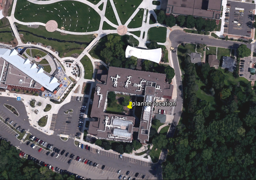Figure 1: The site of this Field project was the courtyard of of the Phillips Science Builiding, located on the lower campus of the University of Wisconsin Eau Claire.

 We as a group conducted our measurements on the morning of January 27th  and we convened at 930 AM and were finished with taking our measurements by 11:40 AM. The conditions got increasingly colder and windier during our time outside.  at the start, the temperature on my mobile phone, a Galaxy Prime made by Samsung, indicated that it was 21 degrees with a windchill of 15.  By the end of our time, the temperature read 18 degrees with a windchill of 8. 

Methods

figure 2: grid created over planter box

The first thing we did in preparation for our measurements is to create our landscape within the planter box.  To do this, my group members and I used our hands and shovels to create varying hills, slopes, ridges, valleys and depressions.  Once we were satisfied with what we had made, we used water from a water bottle help compact the snow surface and freeze the formation in place.  Doing this allowed for us to be less concerned about potentially damaging our landcape accidental as we took our measurements or created our grid. The next thing we did was create our grid, a final product which can be seen in figure 2 blow to the right.  To create this grid, my group members and I decided that it was best to have the x axis be divided into 22 sections and the Y axis into 11 sections.  For both axis's, the divisions were made every 10 cm so that each box covered a square meter. However, because the dimensions of the planter box were not equally divisible by 10, the row on the right side of the box has a y dimension of 12 cm and the column near side had an x dimension of 14 cm ( reference the image in figure 2). otherwise, 210/242 are all the 1 square meter in size. To label the grid blocks, we used a numbering system that began at 0 and when up incrementally by one until the end of the planter in both the X and Y direction.  The point of origin can be seen in figure 2 near the top left of the image. The zero point that we decided for the z value would be the top of the planter.

In terms of collecting heights, my group members and I used two rulers to collect the heights of the surface for each cell. If a cell's surface is below the flush surface of the planter, a ruler was laid on the wood and extended out to the cell and provided a visual place marker on the ruler, showing us how below planter top the surface is.  If the surface was visibly above the planter, the rule used as the visual place marker was held by me as I tried to make it as level possible with the other ruler which was propped up on top of the planter bored to keep.  Where the horizontal met the vertical meter stick, would be the height above the planter the surface was for that cell block.  I did the best i could to keep the horizontal meter stick level and and also tried to measure from the center most of each cell, regardless if it the cells surface was below, above, or level with the edge of the planter.

Results

As we we did our measurements, the figures were recorded in a field notebook.  After that, the numbers were entered into a excel table. This table can be seen in figure 3 below.

figure 3: The numbers in each cell represents the z value of surface in the planter.The redder the lower. The greener the higher.

 
Discussion of Data 

Given the cold conditions, there was some level of haste to this whole operation.  Near the end of the collecting process, everyone was ready to get out of there and were likely working at faster pace, and not being as concise with our measurements.  Also, when collecting the the surface heights of portions that were above the planter surface, bend in the ruler or a poor job of holding the ruler level by me, could have lead us to record figures that were either to low or too high. Going forward, we as a group should consider things like this and alter our methods as such.  I think in the future, on days when the conditions are not good, it would be wise to take breaks inside so that we can stay focused on what we are doing and not not trying to keep adequate warm blood flowing to our hands and feet. Otherwise, suck it up an be ready to face the elements. 

Conclusion

The surface has been made, the data collected, and the results have been discussed, but is this enough?  In the next lab we will learn how to bring this table into an ArcMap Geodatabase, and ultimately conduct geospatial operations on it so that we can better represent the surface we created. by re-creating this project in a digital format, we can then begin to compare and contrast this data collection method with other ones, and see which ones could be more appropriate for similar projects going forward.