Lab 7:Distance/Azimuth Tree Survey: UW-Eau Claire Campus, Phillips North Lawn

Introduction 

Much of the field work that is currently done in the professional geospatial industry is contingent upon the full functionality of the newest, shiniest technology.  The thing is though, with these amazing tools come amazing headaches, and at times the technology can completely  fail the user, and become useless.  When this happens, one must resort to more traditional methods of geospatial surveying to complete the task assigned.  With that being said, the method that will be discussed and demonstrated in this lab does still make use of some electronic technology, it can still be done with tools that are completely independent of electronics/satellite connections.  This method is what is known as a distance-azimuth survey, and it is conducted by taking distance and azimuth degree measurements from a single/known point.  With this information, after a few simple operations in ArcGIS, the locations of what ever it is that is being recorded  can be identified with moderate accuracy.   In the sections that follow, methods and results will be discussed that pertain to a distance azimuth survey that was conducted on Tuesday, April 5th, 2016.  

Study Area

In this particular lab demo, students conducted a distance azimuth survey of trees on the Phillips Science Building's North Lawn.  The study was conducted by the full class, and was guided in part by Professor Jo Hupy.  The surveying began at roughly 325 PM and ended at around 440 PM.  The conditions on that day, April 5th, were cold and damp.  The weather was roughly 35 degrees, with gusting winds and a constant drizzling rain that lasted the entire survey.  The specific area where the survey was an area to the North West of the main body of the Phillips building, and to the North East of the Davies Center building. Cutting through the study area is the Little Niagara Creek, which runs East/West through the campus.  The land on both sides of the creek gradually moves from more consistent level ground, into a gradual slope as the land approaches the creek.  Trees were surveyed from both sides of the creek.   The point from which data was recorded was on the south side of the creek. At the time of the Survey, there was heavy foot traffic as students were coming and going from their classes, the atmosphere was someone chaotic and high paced as many were trying to escape the damp and cold.  

The point that anchored this distance azimuth survey was anchored by a man made crack that was created as a gap between slabs of concrete on the sidewalk, directly adjacent from a light pole.  The light pole was intended to be the anchor point of this distance azimuth survey, but was changed to the crack because at its widest point, allowed for people to stand unobstructed by the pole. The crack was roughly a foot and a half long, on one side was grass and on the other side, a complete concrete slap. This was useful because one could place there feet at the edges of the crack, with their toes behind crack, and make consistent measurements from the same point.  Below, in figure 1, one can see the general layout of the study area.  It should be noted, however, that the trees shown in this map do not highlight any part of the trees that were used as apart of this survey. 

figure 1: Study Area for Distance Azimuth Tree Survey.

Methods - Part 1: Collecting Tree Data 

To conduct this survey, the class needed to record three things in pertaining to each tree. The distance from the anchor point in meters, its azimuthal location on a scale of 0 to 360 from the anchor point, the trees common name, and the diameter of its trunk. The distance measurements were taken by two separate devices.  One device was a pulsating device which recorded distances based off of sound pulse that was originated at the anchor point and traveled to the tree where another student was holding a counter part of that device, which than deflected the sound back to the main device.  Given that the speed of sound is relatively constant, the time between when the pulse leave the device, bounces off of the the counterpart, and returns, providing a distance value between the the observation point and the tree. This distance provides distance and distance alone.  However, the second device, which makes use of a laser and an internal compass, provides both a distance and an azimuthal direction. 

In terms of measuring the width of tree trunks, this was done with a simple measuring tape with a hooked end. The hooked end allowed for the measures to stick the tip into the wood, where it remain steadfast in the bark, while the rest of the tap could be rapped around the trunk to record the distance. The identification of the tree was done by relying on the good judgement of the professor.  

Since the class was all recording the information individually, there needed to be someone to relay the information  from the the party that was conducting the tree girth measurements and species types, to the others by the anchor point. After about two tree measurements, the two students that were accompanying the professor would switch out, and the two that were previously with the professor would join the others.  This ensured that everyone would would have experience with all components of the equipment.

Once professor Hupy dubbed the survey complete, students than returned inside so that the classcould record the data into a digital format in ArcMap.

Part 2: Creating Data in ArcMap

Now that the dataset has been created of trees in the Phillips North Lawn, the class can now input this data into an excel table so that it could be turned into features and eventually mapped.  Figure 2 below shows the table that was made. 

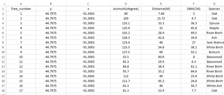figure 2: table that was made in Excel from data collected in the field.  The X and Y field are all the same values because that represents the anchor point 

Once the data was in this digital format, it could then be turned imported into a geodatabase in ArcMap and be transformed into a recognizable set of features, relative to the data that was mapped.  With that, now the workflow will be laid out as to how to create the features desired from this survey.

1. Using the Barring Distance Line Command, input the table and populate the X, Y, Distance, and Bearing fields appropriately. 

2. The output of this operation will be the lines at the appropriate distance and bearing from the anchor point, as seen in figure 3 below.

figure 3: output of distance to line tool

3. Now that this feature has been created, students were to use the feature vertices to point commands to create the endpoints at these lines that represented the tree locations. 

4. Within this tool, the input needs to be the feature that was previously created using the barring distance line tool. 

5. VERY IMPORTANT - change the option at the bottom titled "point type" from 'all', to 'end'. Doing this populates the outputted field with the right number of points.  Leaving this option as all will create two points, one at the beginning and one at the end. 

figure 4: output of feature to vertices to point tool

6. The output of this tool will create the point locations of the tree locations. figure 4 to the right shows these points, with out the lines which provided them. 

7. Now the feature that were desired have been created,  however, the fields associated with these features are not complete.  This point field does not have the species or tree width attributed to the original data. 

8. To complete this feature, it will be necessary to conduct a table join with a table that contains this information.  The join for this field should be based of off Tree_Number.

9. Export the feature to make the join permanent.  The best place to export the feature to is the geodatabase that has been used prior.

10 (optional).  If publishing these feature to web service, project the feature to web mercator.  

Once this is complete, the final feature is a point location with all the data that was recorded at the initial onset of this survey.  

Results and Discussion 

Below is an embedded map that shows  the results of survey.  The point locations visible are tree locations.

as you can see, there are some clear discrepancies in the location of these trees.  This is likely as result of human error, since most of the class had never conducted a survey such like this, let alone work with the equipment ever before.  It is more than likely that somewhere in the process, one, if not all of the students made an error in producing the data with the equipment at hand.  In that sense, this lab could be viewed as a disappointment. However, looking past these errors, with more practice and experience on individual levels, this sort of skill set could be very useful in the future, for it is never easy to predict when and where technology will fail.    

Conclusion

A distance/azimuth survey is handy skill for any survey technician, GIS specialist, or all-purpose-geographer to have in the toolkit.  In this day in age, technology is a crutch that we tend to depend on very heavily, often to a fault.  When it fails, there is a tendency for users of the technology to give up and say today is not my day, and wait for the technology that was intended to be used in the survey to be available for use again.  This is sometimes necessary, but if able one could consider using this method to save the the time that it would take to leave the sight , fix the equipment, reorganize and return to the field sight.  Being able to operate with lower grade technology is a skill in itself, and this is just one example of how it can be helpful